Traditionally Microsoft Excel has covered the majority of formulas any aspiring PPC superstar could want. However that gap is widening and now (more than ever perhaps) it is worth looking at some additional functions and formulas available only in Google Sheets. We have picked our top 5 PPC formulas exclusive to sheets. Which one do you like best, are you going to use next or what have we missed? Be sure to add in the comments underneath!
1) Deduplicate rows of text both quickly and on the fly using the UNIQUE formula
Deduplicating rows of text is made easy with the UNIQUE function. In essence it is the formula based route to removing deduplicates through the data section of Excel & Google Sheets. The benefit of this approach comparatively rests in its scalability. If every time in Google Sheets we have to go (Data menu > Data Cleanup > Remove Duplicates) its a manual process. Pulling in unique can help find unique search queries and much more.
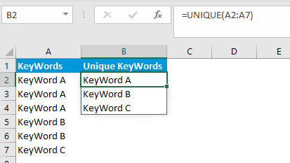
- In the below we have a list of keywords in column A. Spanning rows 2 to 7
- We add in the UNIQUE formula in another cell – in this example below cell B2. Copy and paste the formula below.
=UNIQUE(A2:A7) 
To enhance the scalability here you can apply to the entire column as below
=UNIQUE(A:A) 2) Use the IMPORTRANGE formula to add in data from another Google Sheet
This is something we use quite regularly. Particularly if there is a requirement for data to be gathered from a multitude of sheets.
To use the IMPORTRANGE range formula. The formula includes 3 parts:
- The spreadsheet URL
- The tab name followed by an exclamation mark
- The range
=importrange("https://docs.google.com/spreadsheets/d/1N4emko8yHFU0EYIdlBczNKOiW939VdIWZl_URnmFPpM/edit", "Budgets!B2:B2")
3) Try the SPARKLINE Google Sheets formula to add basic time series charts in a single cell
Sparkline charts may be simple but they are super effective. This is possible within Microsoft Excel but not instantly as a formula. To add the most simple of sparkline charts just use this formula
=SPARKLINE(A27:D27)
4) Use the SPLIT formula for separate text to columns
Within a lot of campaign / ad group naming conventions different breakouts are often separated by a hyphen – or bar | (the delimiter) . Whilst both Google Sheets and Microsoft Excel have a function for separating text to columns – Google Sheets also handily has a formula to achieve the same result. To use SPLIT…
=split(A2,"|")5) Load in the QUERY formula in to only show the highest items in a set of data
This is a little more difficult as it includes a query to perform written in Google Visualization API query language. Rest assured its not complicated when you get your head round it! You can also just take the below and just change what you need. If you get stuck just add a comment and we can help!
=QUERY(A:E,"SELECT A,C Order By C Desc Limit 5")In the above example
- The A:E part just designates the table or column names with the data you want
- the Select A part simply shows that we are looking to return the keyword (eg in column A)
- The C Order By C is showing that we want to capture the cost which is column C whilst also ordering by this column too
- The Desc Limit 5 caps the number of items returned to 5

In Summary
Sometimes is not about picking one or the other (eg Google Sheets vs Microsoft Excel). But having awareness around exclusive formulas and functions will help make picking the right platform for each task! Which of the above did you like most? Did you get stuck? Drop in a comment below to let us know what you think, what you found useful or what your favourite Google Sheets only formula is

